Two Methods of Conditional Generation

tldr; There are two main ways of doing conditional generation using deep generative models, the activation maximization approach and the latent variable approach. These two ways correspond exactly to the two different ways a joint distribution can be factorized. We introduce these two basic methods and combinations of them.

A generative model describes the joint probability distribution \(p(x,c)\) for data point \(x \sim X\) and condition \(c \sim C\).

Suppose we wanted samples from a generative model meeting certain conditions. For example, if \(X\) was the set of faces and \(C\) was a variable measuring facial beauty, then there are two main methods we can use if we wanted to sample from the set of pretty faces.

These two methods correspond exactly to the two different ways the joint distribution can be factorized.

Activation Maximization Approach

In the first approach, we factorize the generative model \(p(x,c)\) into the discriminator for the condition \(p(c|x)\) and the data generator \(p(x)\).

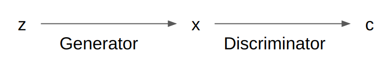
The naive (but expensive) way to obtain pretty faces is to sample from the generator repeatedly and discard all the faces that the discriminator says are not pretty.

Where the generator \(G\) is a deep neural network, we can update its parameters so that it only generates pretty faces. This can be done by updating it along the direction of \(\nabla_G c\) to maximize the activation of \(c\). This activation maximization based approach is also known as a plug and play generative network¹.

The generator can be trained separately from the discriminator, which is helpful in semi-supervised settings, where we might have far more unlabelled data than labelled data.

Incidentally, a generative adversarial network follows this approach, where \(C\) corresponds to the realness of the data.

Latent Variable Approach

In the second approach, we factorize the generative model \(p(x,c)\) into a prior on the condition \(p(c)\) and a conditional data generator \(p(x|c)\).

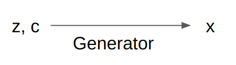
To obtain pretty faces, we simply have to set a fixed \(c\) while sampling \(z\) from the latent space \(Z\).

There are multiple ways \(z\) can interface with \(c\), but ideally, we would like to learn a disentangled latent representation so that we can control the generative process only along the dimension of \(C\) without changing any other properties of the data.

This method is especially useful when the problem domain gives us a useful prior on \(c\) or when the data generating process might differ significantly depending on what \(c\) is.

Combination Approaches

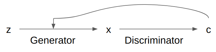
It is also possible to combine the two approaches, by starting with the Activation Maximization approach (using an initial prior for \(c\)) and then feeding \(c\) back in as a latent variable for the generation process. An example of this can be found in Toward Controlled Generation of Text. Hu et al.

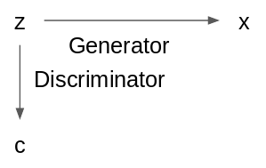
In Latent Constraints: Learning to Generate Conditionally from Unconditional Generative Models. Engel et al., the authors trained a condition discriminator on the latent code \(z\) itself rather than data point \(x\). This allows us to shape \(z\) itself without having to backpropagate through \(x\), which is useful when \(x\) is discrete.

In general, it does not seem like any one approach is obviously superior to any other approach. Picking the right approach is therefore highly problem and architecture dependent.